Plotting with stemtools • stemtools

This vignette showcases every plotting function in stemtools: stem_barplot(), stem_barstack(), stem_inline(), stem_battery() and stem_multiselect(). We’ll use the simulated trust dataset that ships with the package.

library(stemtools)
library(ggplot2)

data(trust, package = "stemtools")
head(trust)
#>                       police                 government
#> 1 Neither Agree nor Disagree            Rather Disagree
#> 2           Definitely Agree        Definitely Disagree
#> 3           Definitely Agree        Definitely Disagree
#> 4 Neither Agree nor Disagree            Rather Disagree
#> 5 Neither Agree nor Disagree Neither Agree nor Disagree
#> 6           Definitely Agree Neither Agree nor Disagree
#>                           eu                army                 scientists
#> 1 Neither Agree nor Disagree    Definitely Agree Neither Agree nor Disagree
#> 2 Neither Agree nor Disagree        Rather Agree            Rather Disagree
#> 3               Rather Agree    Definitely Agree            Rather Disagree
#> 4            Rather Disagree    Definitely Agree Neither Agree nor Disagree
#> 5 Neither Agree nor Disagree    Definitely Agree               Rather Agree
#> 6 Neither Agree nor Disagree Definitely Disagree Neither Agree nor Disagree
#>      eu_index   nat_index age         W biggest_concern1 biggest_concern2
#> 1    Likes EU     Neutral  41 0.6452540     Unemployment     Unemployment
#> 2     Neutral   Satisfied  38 0.1800867      Immigration       Corruption
#> 3    Likes EU Disatisfied  39 0.2939668      Immigration       Healthcare
#> 4     Neutral     Neutral  34 0.8033685      Immigration       Healthcare
#> 5    Likes EU   Satisfied  41 0.3471653       Healthcare     Unemployment
#> 6 Dislikes EU Disatisfied  35 1.2082489      Immigration       Healthcare
#>   biggest_concern3
#> 1      Immigration
#> 2      Immigration
#> 3       Corruption
#> 4       Corruption
#> 5      Immigration
#> 6       Corruption

Setting the Stem theme

theme_stem() is a complete theme carrying the Stem look. Because it is complete, the plotting functions do not apply it themselves – instead we switch it on once with theme_set() and every plot from here on picks it up automatically:

theme_set(theme_stem(family = ""))

We pass family = "" so the plots fall back to the graphics device’s default font (the Stem house font, Calibri, may not be installed on every machine). In normal use you would just call theme_set(theme_stem()).

How the plotting functions are built

All the plotting functions are composed from a shared frequency core. Each one calls stem_summarise_cat() to compute (possibly weighted) proportions with 95% confidence intervals, then hands the aggregated data to a ggplot2 template. You can call the frequency function directly whenever you need the numbers themselves:

stem_summarise_cat(trust, item = police, group = eu_index, weight = W)
#> # A tibble: 20 × 5
#>    eu_index     police                       freq freq_low freq_upp
#>    <fct>        <fct>                       <dbl>    <dbl>    <dbl>
#>  1 Likes EU     Definitely Agree           0.395   0.327     0.463 
#>  2 Likes EU     Rather Agree               0.318   0.251     0.384 
#>  3 Likes EU     Neither Agree nor Disagree 0.149   0.104     0.194 
#>  4 Likes EU     Rather Disagree            0.0643  0.0264    0.102 
#>  5 Likes EU     Definitely Disagree        0.0734  0.0346    0.112 
#>  6 Neutral      Definitely Agree           0.405   0.330     0.480 
#>  7 Neutral      Rather Agree               0.312   0.242     0.383 
#>  8 Neutral      Neither Agree nor Disagree 0.178   0.117     0.239 
#>  9 Neutral      Rather Disagree            0.0637  0.0297    0.0978
#> 10 Neutral      Definitely Disagree        0.0406  0.00841   0.0728
#> 11 Dislikes EU  Definitely Agree           0.400   0.305     0.495 
#> 12 Dislikes EU  Rather Agree               0.326   0.234     0.418 
#> 13 Dislikes EU  Neither Agree nor Disagree 0.155   0.0778    0.233 
#> 14 Dislikes EU  Rather Disagree            0.0368  0.00956   0.0640
#> 15 Dislikes EU  Definitely Disagree        0.0819  0.0190    0.145 
#> 16 Doesn't Know Definitely Agree           0.308   0.191     0.424 
#> 17 Doesn't Know Rather Agree               0.453   0.315     0.591 
#> 18 Doesn't Know Neither Agree nor Disagree 0.180   0.0871    0.272 
#> 19 Doesn't Know Rather Disagree            0.0139 -0.00215   0.0300
#> 20 Doesn't Know Definitely Disagree        0.0455 -0.00160   0.0926

Every plotting function accepts the same core arguments:

item – the categorical variable to plot,
group – an optional grouping variable,
weight – optional survey weights (passed to surveycore),
palette and direction – the Stem colour palette to use,
label_* – controls for the percentage labels.

Simple bar plot

stem_barplot() draws the distribution of a single categorical variable as horizontal bars, one bar per category.

stem_barplot(trust, item = government)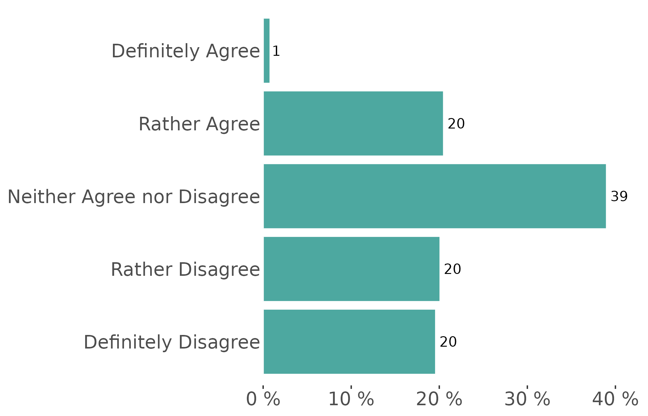

Confidence intervals are always computed and can be shown with errorbar = TRUE.

stem_barplot(trust, item = government, errorbar = TRUE)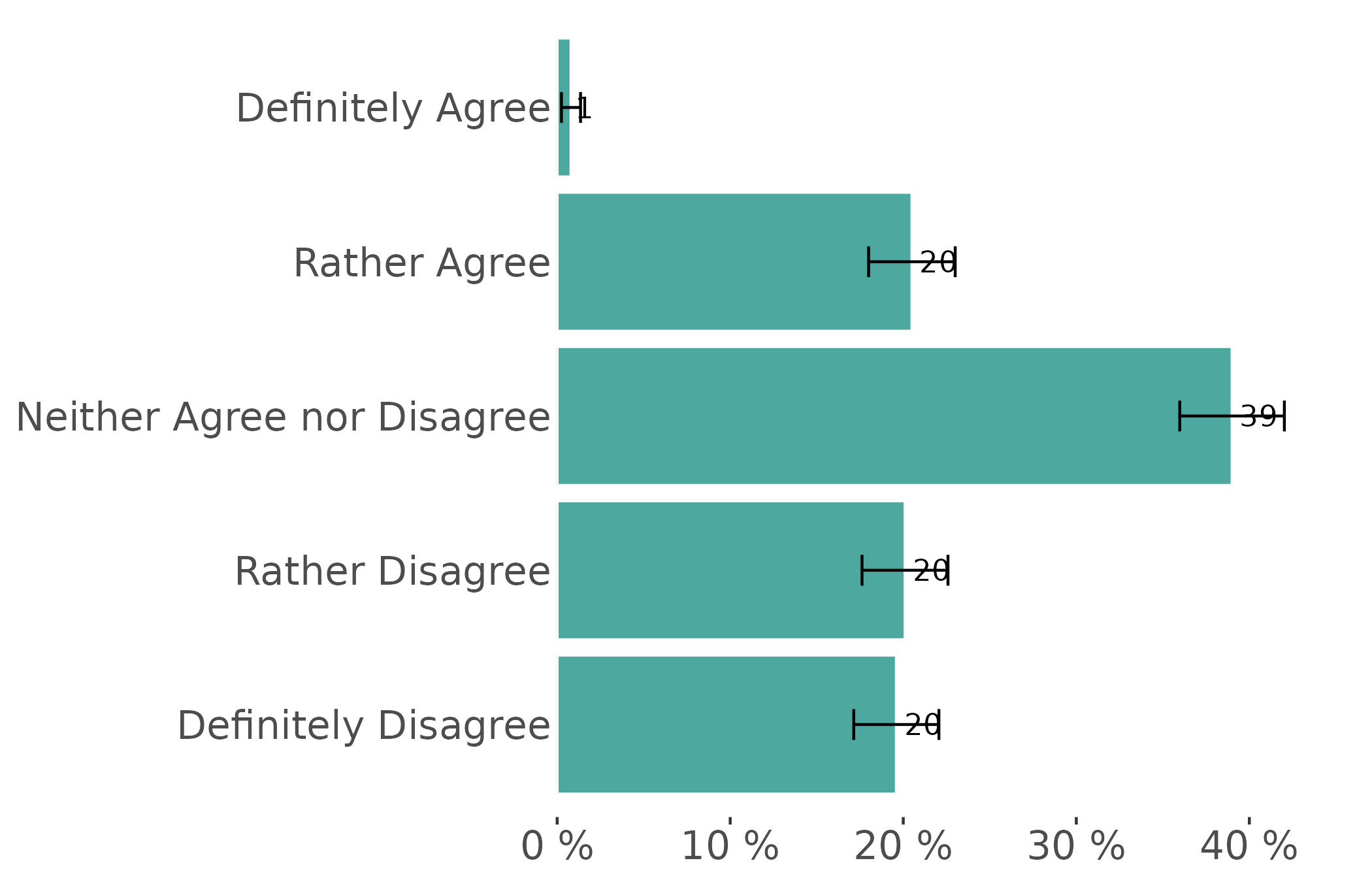

Supplying a group variable instead draws one stacked horizontal bar per category of the group, with the item mapped to fill. Proportions are computed within each group, so every bar sums to 100%, which makes it easy to compare the composition of the item across groups.

stem_barplot(trust, item = police, group = eu_index, weight = W)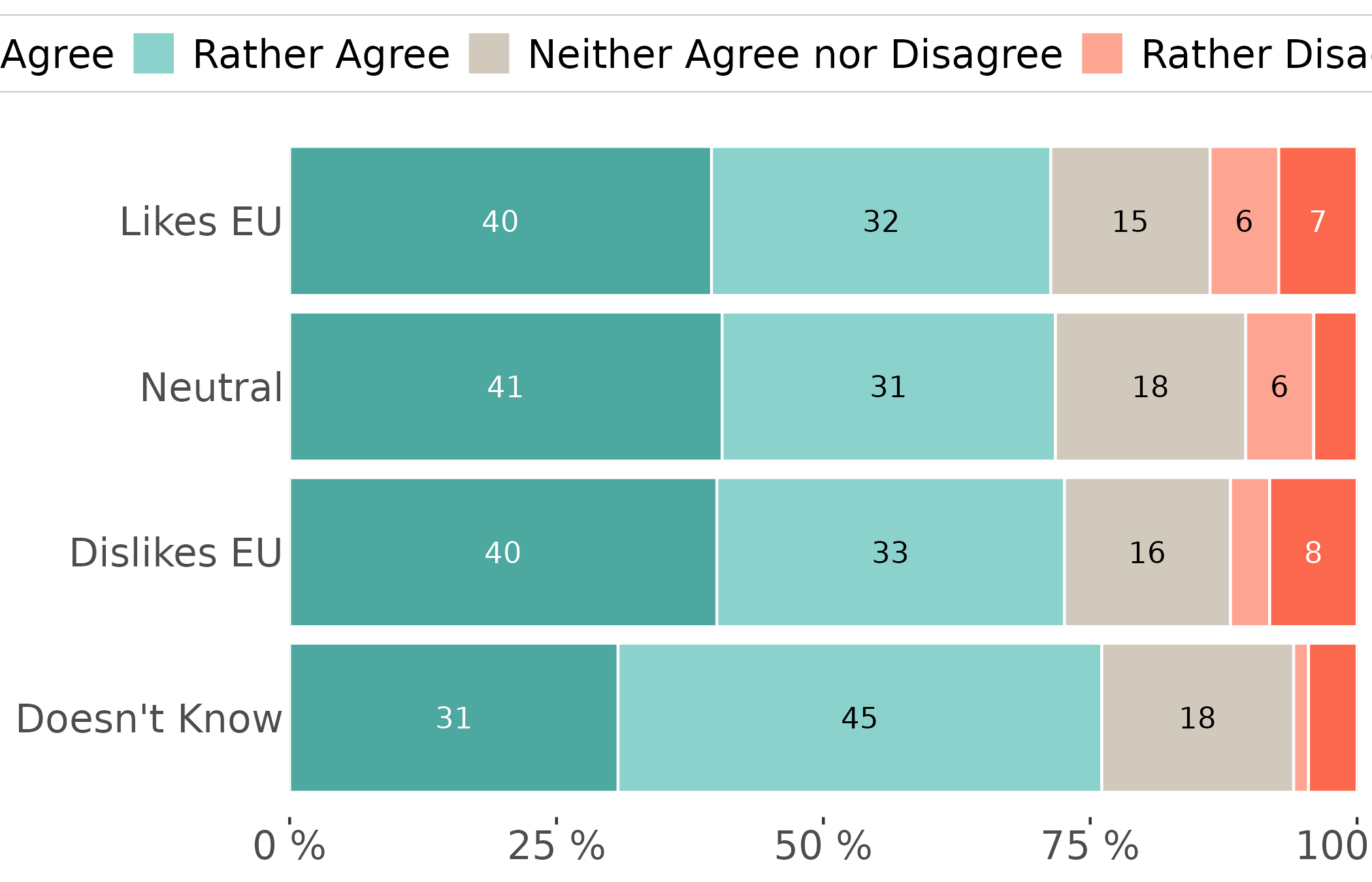

Inline bar plot

stem_inline() is a compact summary of a single variable as one stacked horizontal bar.

stem_inline(trust, item = police, weight = W)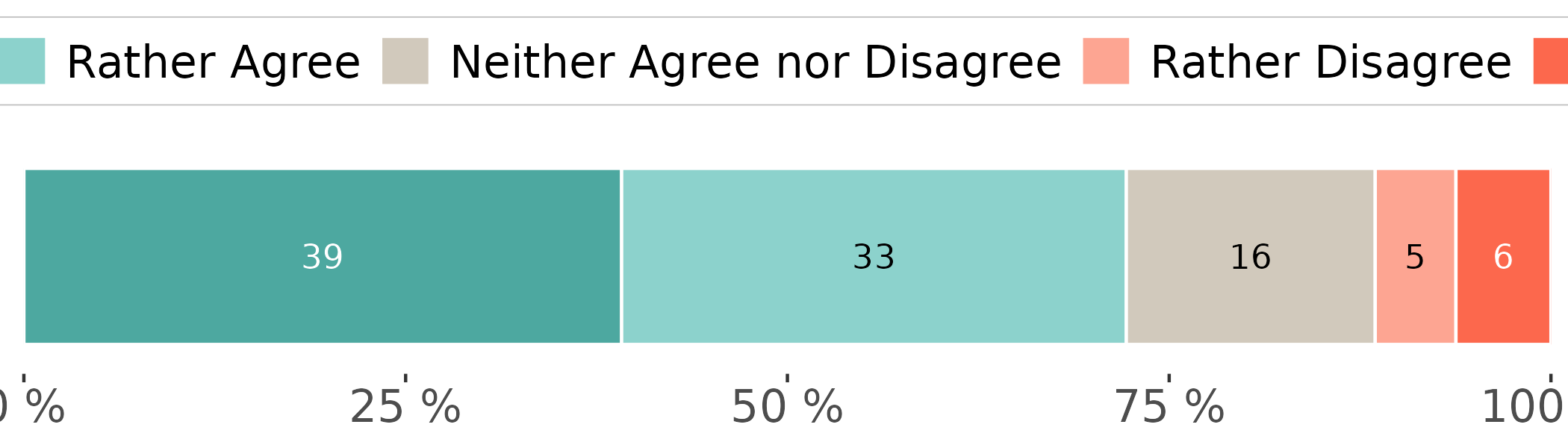

Battery of like items

stem_battery() plots several variables that share the same response categories (a Likert battery, say) as one chart, with a stacked bar per item. Pass the items with tidyselect helpers and, optionally, order_by to sort the items by their combined share of one or more categories.

stem_battery(trust,
             items = c(police, eu, government, army, scientists),
             weight = W,
             order_by = c("Definitely Agree", "Rather Agree"))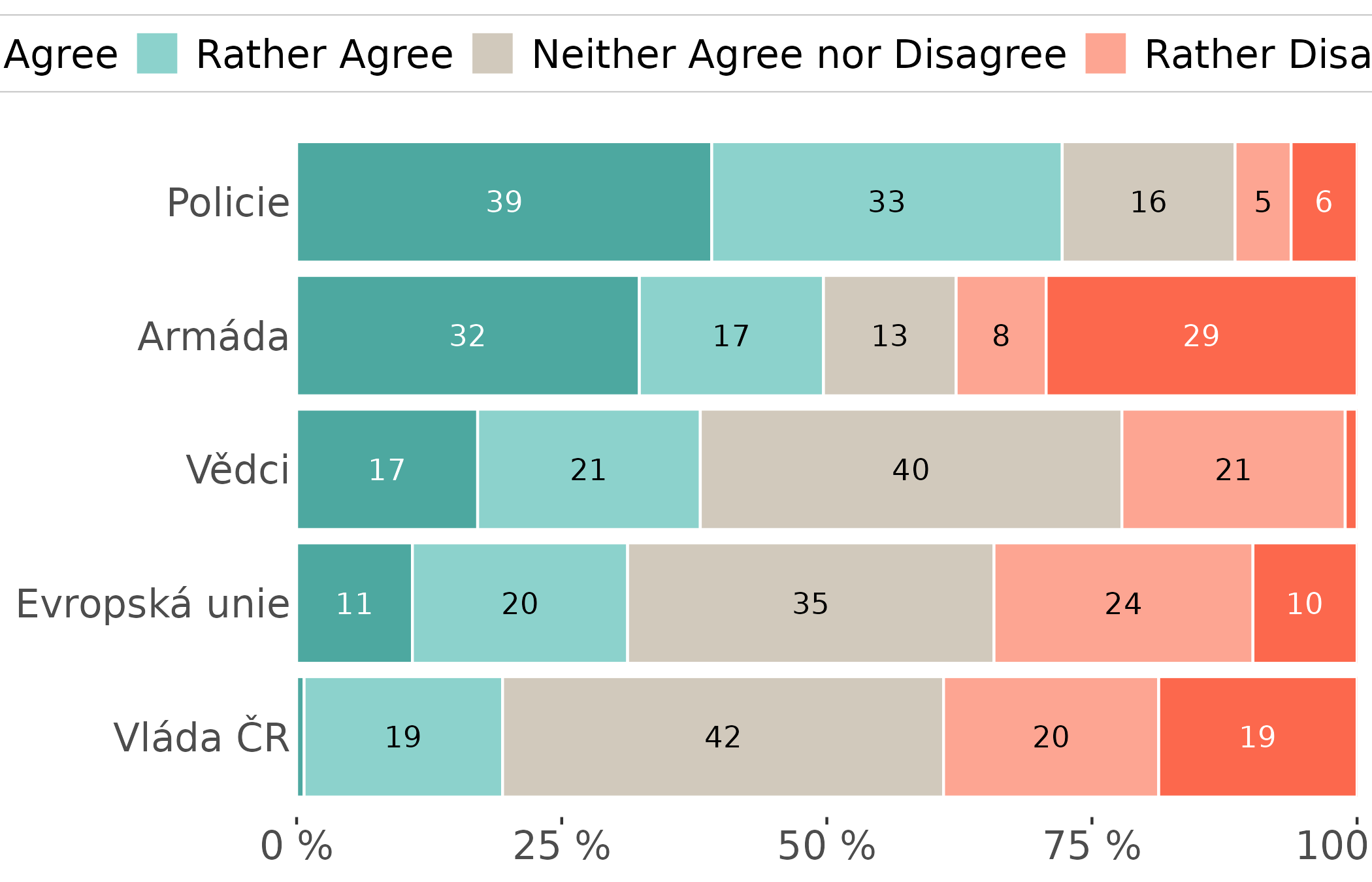

Item labels (the "label" attribute) are used automatically when present; set item_label = FALSE to use the bare variable names.

Multiple-choice items

stem_multiselect() summarises a set of “select all that apply” items, rescaling the frequencies so the bars show the share of respondents who picked each option (rather than the share of responses).

stem_multiselect(trust, items = dplyr::starts_with("biggest_concern"), weight = W)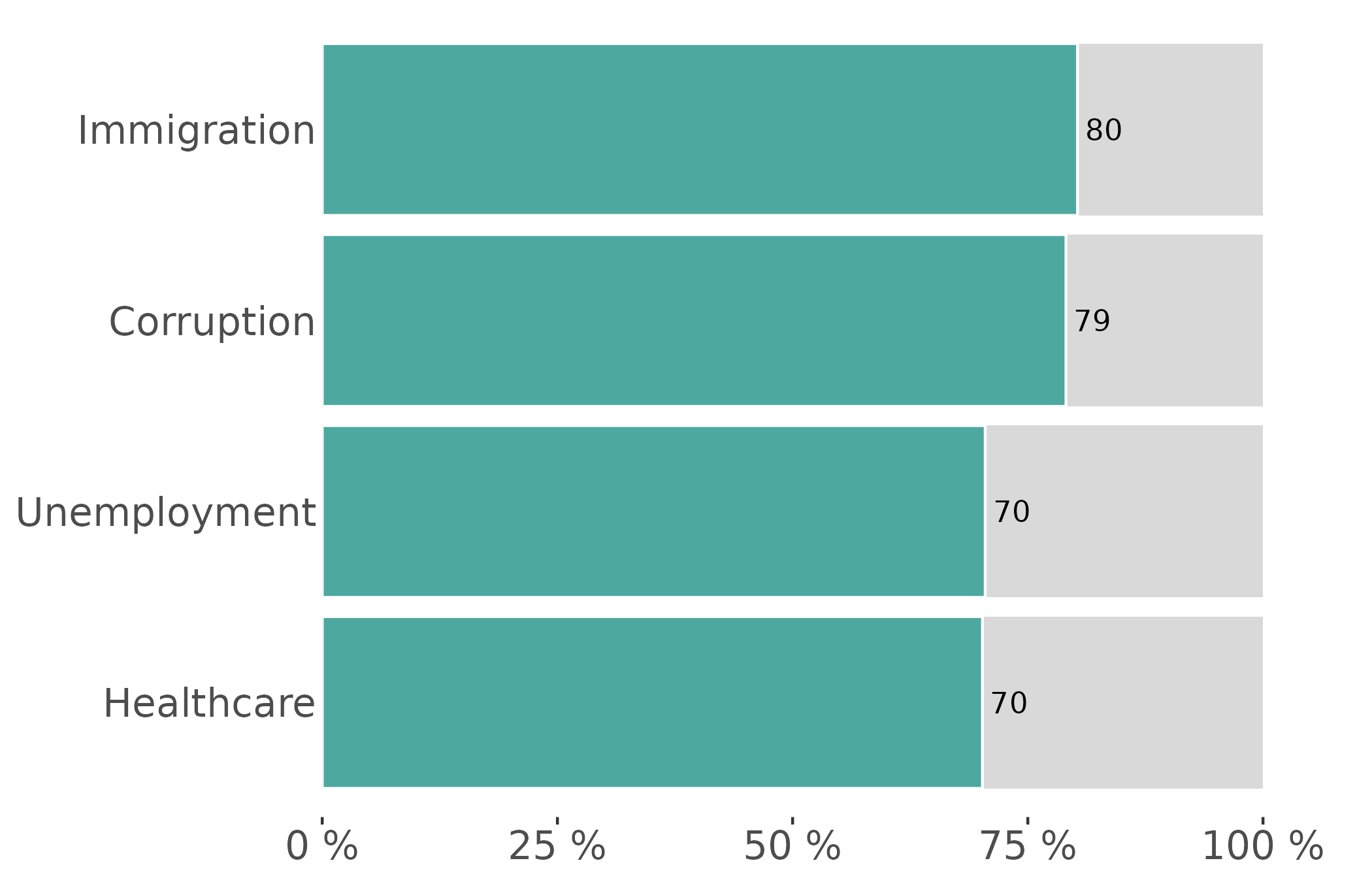

Supplying a group variable draws dodged bars for a within-group comparison.

Customizing labels

By default the plots print a percentage label on each bar (set labels = FALSE to hide them). label_accuracy controls rounding (1 for whole numbers, 0.1 for one decimal place), label_suffix sets the text appended to each label and label_hide suppresses labels for proportions below a threshold.

stem_barplot(trust,
             item = police,
             group = eu_index,
             label_accuracy = 0.1,
             label_hide = 0.1)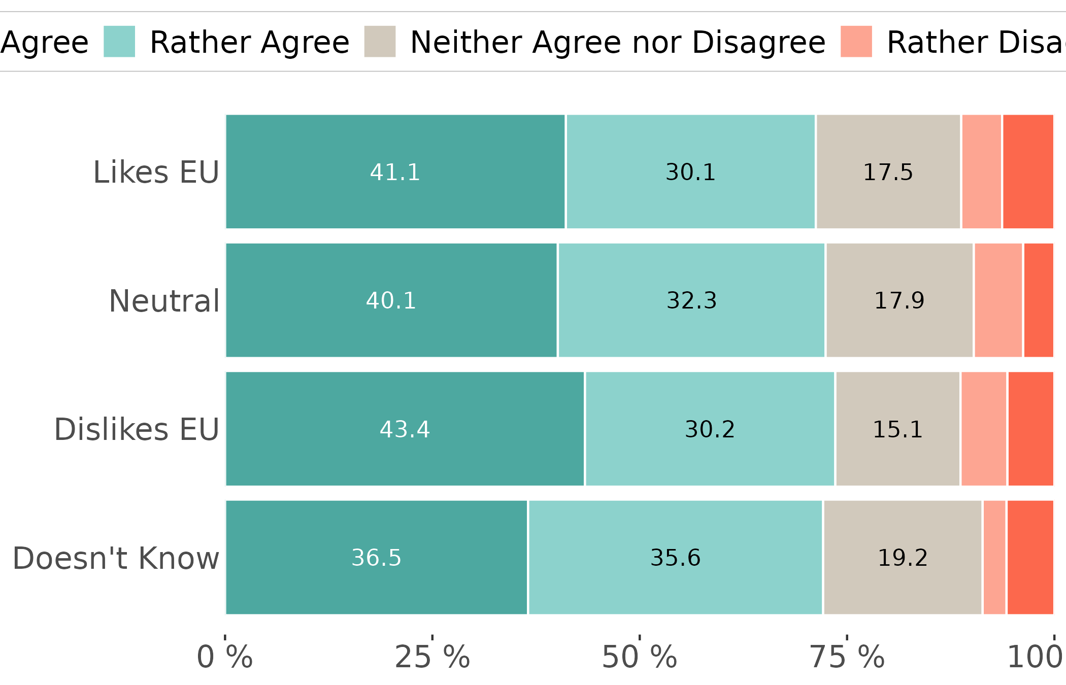

Colours

Use palette to pick one of the Stem palettes and direction = -1 to reverse it.

stem_barplot(trust, item = police, group = eu_index, palette = "div2")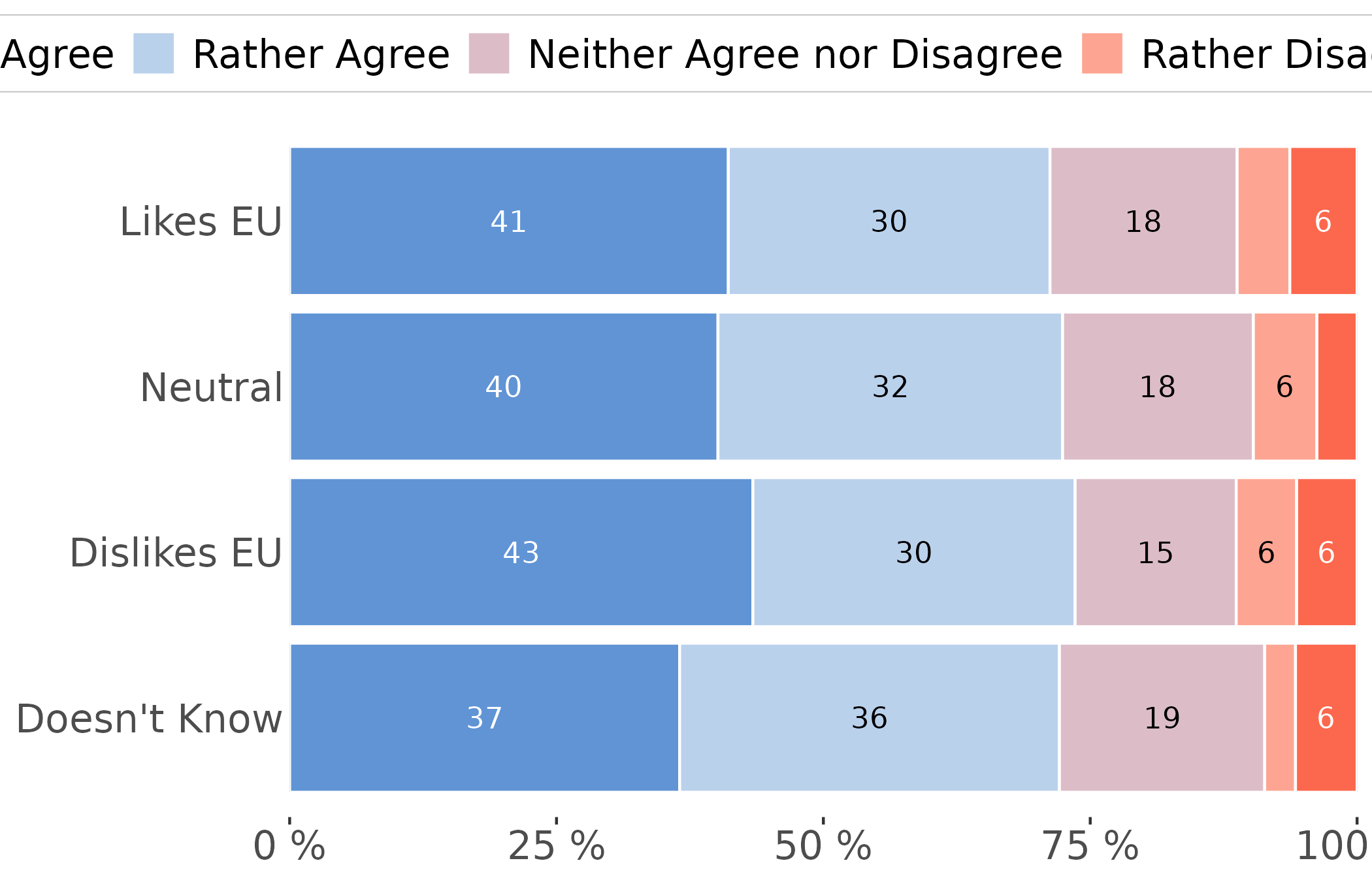

Collapsing categories

collapse_item and collapse_group collapse (or rename) categories by passing a named list, exactly as in stem_summarise_cat().

stem_barplot(trust,
             item = police,
             group = eu_index,
             collapse_item = list(`Ano` = c("Definitely Agree", "Rather Agree"),
                                  `Ani ano, ani ne` = "Neither Agree nor Disagree",
                                  `Ne` = c("Rather Disagree", "Definitely Disagree")))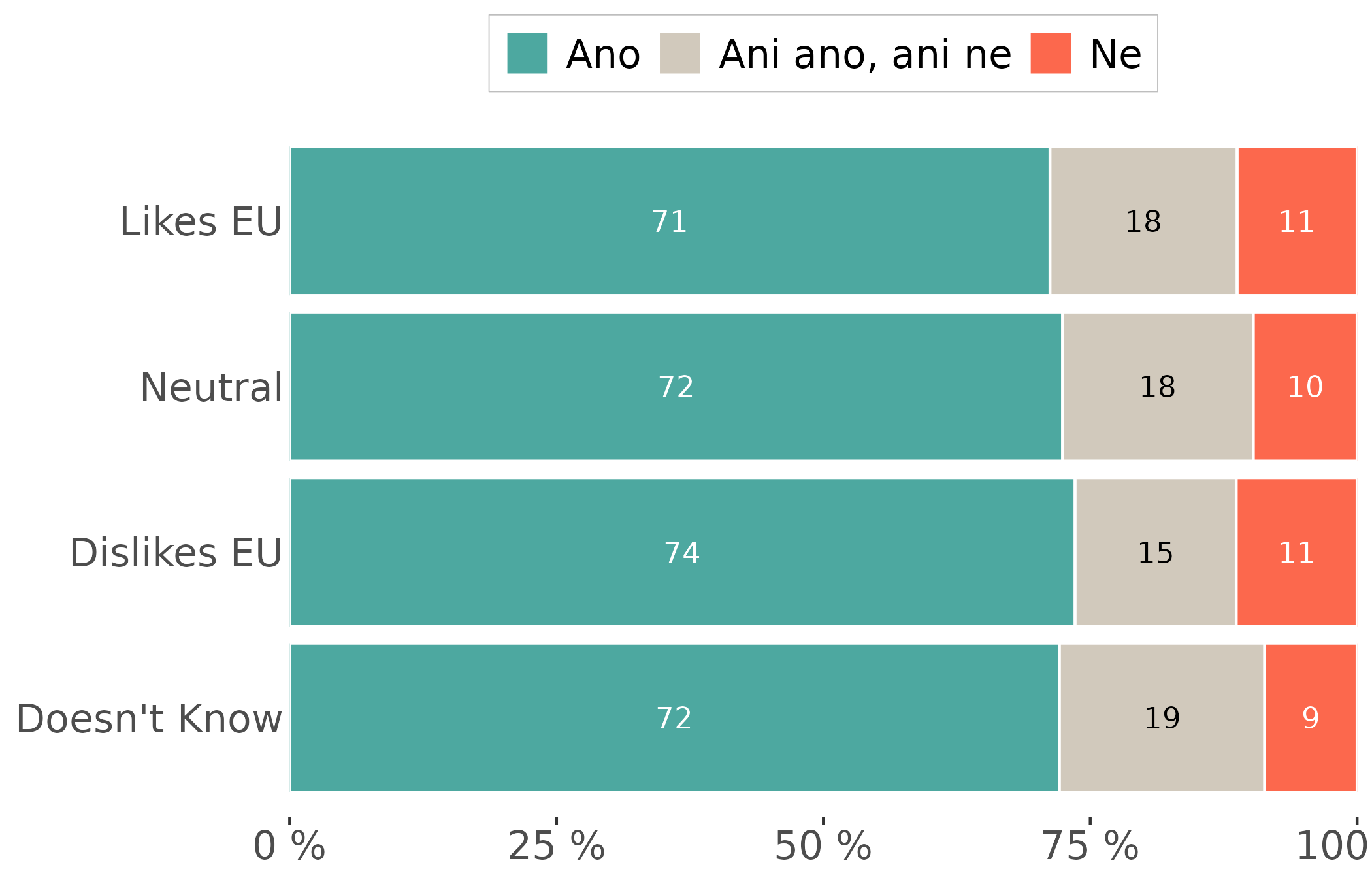

Weights

If a weight variable is specified, weights are treated as survey weights and passed into surveycore, which builds a Taylor-series survey design. Manipulating that design uses surveytidy, whose verbs mirror dplyr, so weighted and unweighted code read the same way.

With unweighted data, the confidence intervals are computed using the basic $\sqrt{\frac{p \cdot (1-p)}{n}}$ formula. With very small proportions and small samples this can lead to bounds outside of the (0, 1) range. With weighted data, the confidence intervals come from surveycore using Taylor-series linearization.

stem_barplot(trust, item = government, weight = W)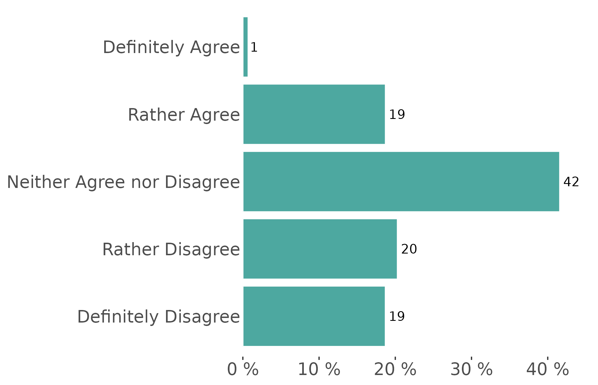

Further customization

Every function returns a standard ggplot2 object, so you can keep adding layers, scales and theme tweaks. The global theme_stem() is already applied, so this just layers a title on top:

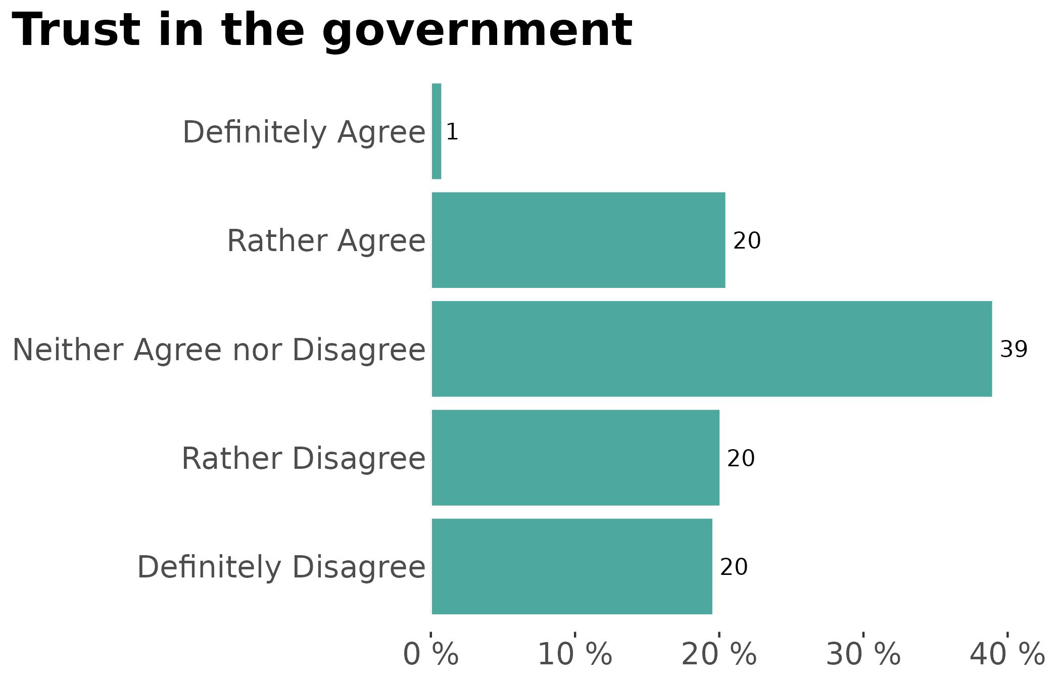
stem_barplot(trust, item = government) +
  labs(title = "Trust in the government")